
GA Approach to Small Transmitting Loop Design
Designing Electrically Small Loop Antennas with Modern Numerical Methods
Matt Roberts - matt-at-kk5jy-dot-net
Updated: 2017-02-01
Introduction
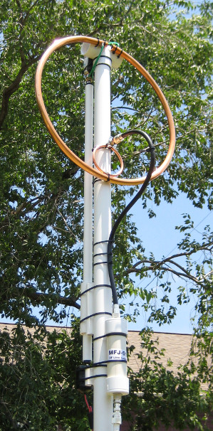 This is a companion project to my small transmitting loop experiments.
Those experiments have produced a number of loop antennas of different sizes and configurations,
and have demonstrated to my satisfaction that the small transmitting loop can be a serious HF
antenna system.
This is a companion project to my small transmitting loop experiments.
Those experiments have produced a number of loop antennas of different sizes and configurations,
and have demonstrated to my satisfaction that the small transmitting loop can be a serious HF
antenna system.
Designing such an antenna involves balancing a number of variables, such as overall size, shape,
conductor diameter and material, capacitor voltage and current ratings, desired power handling,
and of course the desired frequency range. Some of these variables are critical in the
sense that small changes in their values can lead to large changes in the performance of the
antenna for any given frequency. As such, any such antenna is a compromise between these
variables. When a loop is intended for use on more than one band, it can be difficult to
find the right combination of measurements that will optimize the antenna such that it is the
best compromise across the intended bands of operation.
These design challenges prompted me to look for ways to automate the design process, so that I
could select which characteristics are important to me, and allow a computer to determine the
details to make the best overall antenna for the constraints I provide. This has led me
to experiment with a tool I first encountered in graduate school --
Genetic Algorithms.
GA: The Quick Summary
The Wikipedia article linked above provides a better explanation of the so-called "genetic
algorithms" than I could repeat here. I would summarize these tools as a way to do
automated experimentation, testing and optimization of potential solutions to problems
that can be modeled with a computer. GAs are part of a larger family of techniques known
as evolutionary computing,
but there is really nothing "evolutionary" or Darwinian about these techniques.
The so-called genetic algorithm is simply a way for the computer to experiment with different
combinations of primitives, using some very specific criteria that the user (me) provides to
it for determining how "good" a given solution is. Rather than the user having
to find a set of equations that describe the optimal solution, the user only has to provide a
way to measure any given solution. The machine then uses its plentiful and inexpensive
computational time to run experiments on different combinations of features, comparing each
combination with the test criteria, and sorting out the better solutions from the lesser
ones. This approach isn't Darwinian, because every GA problem requires that the user
introduce intelligent input by formulating the selection criteria, but because the original
work sought to emulate Darwin's theoretical process, we are stuck with the name.
In this context, I am using a GA to generate and test different loop antenna designs, to
optimize a single antenna for use on one or more bands. In this way, I don't need to
formulate the best antenna parameters, but I do need to provide the computer with
functions that can be used to compare one design with another. The computer will do
the experiments to generate a large number of antenna designs, then use my functions to
compare them. In GA-speak, these functions together are used to form what is known
as the "fitness function". Rather than sitting a t a computer trying
different combinations of numbers in AA5TB's loop design spreadsheet (which is a
very powerful tool, by the way), I can let
the computer do hundreds of experiments in a second or two, and then give me the best answer.
Where this approach really shines is when solving problems where it is impossible or
impractical to devise a system of equations to solve for an optimal solution, but where
there is a measure for comparing different designs to determine which is the closest to
the desired optimal solution. In these types of problems, the GA can be essentially
another form of numerical computing, determining a solution that is "good enough"
for the needs of the user, without requiring a rigorous mathematical approach to the
solution.
The Fitness Function
The core of any GA is the fitness function. This function is used to measure each
proposed design generated by the GA, and is used to filter or "weed out" the
less useful designs in favor of those with better characteristics. In the first draft
of these experiments, I have chosen a very simple fitness function, which is a product of
four even simpler functions, evaluated together for a specific target frequency, f0:
fitness = [ Efficiency * Bandwidth * Smallness * Conductor ]
where:
Efficiency is a number between 0.0 and 1.0, describing the efficiency
of the antenna. An ideal lossless antenna results in an
efficiency of 1.0, where a pure non-radiating load has an efficiency of 0.0.
Bandwidth is also a number between 0.0 and 1.0, describing the normalized bandwidth,
such that bw(normalized) = bw(Hz) / f0.
Smallness is also a number between 0.0 and 1.0, describing the
electrical smallness of the antenna; 1.0 is an ideally small antenna, and 0.0 is a loop
with a circumference of 0.25 wavelength or more.
Conductor is also a number between 0.0 and 1.0, describing the
reasonability of the conductor diameter; an infinitely small conductor is 1.0, and a
conductor with diameter == 0.1 of the loop diameter is 0.0. This causes the GA
to balance the other parameters with the size of the conductor; otherwise, the GA would
opt for the biggest conductor it could in every design.
This function tries to maximize all four of these items in a resulting antenna design,
and it treats all of them as roughly equal in priority.
The GA generates hundreds or thousands of antenna designs, and uses this overall function
to evaluate each design for each of the bands or frequencies I request. The GA
proceeds through several "generations" of designs, and between each generation,
it attempts to improve the next generation of designs based on the results of the current
generation. In the end, if the GA is configured properly, the final generation
should consist of several designs that are all close to convergence on a single set of
design numbers that I could use to build the best-fit antenna for the constraints
I have provided.
Example Results
The fitness function described above has produced several reasonable antenna designs.
The quality of the results depends on the constraints provided, as with any GA. But
here are a couple of examples that were computed using a generation size of 100 and a limit
of 65 generations, at which time the GA had largely converged to a single preferred solution.
For those of you fluent in GA/GP/EC techniques, the genome was a floating-point vector of
size two, and each of the floating-point numbers in the vector represents a specific measurement
in the antenna design; the first is the overall loop diameter, measured in feet, and the second
is the loop conductor size, measured in inches. Each individual generated is represented
by this pair of numbers.
Loop 1: Single Band, 40m, f0 = 7.1 MHz
The algorithm generated a 40m-only circular copper loop that was optimized for that band
as described above. The loop diameter recommended by the GA was 7.87 feet,
and the conductor diameter recommended was 1.9 inches.
According to the equations taken from Chapter 5 of the ARRL Antenna Book, this antenna will
have an overall efficiency of 85.5% (less than 1dB of conductor loss), a +/- 3dB bandwidth
of 12.7kHz, and when driven with a 100W CW transmitter it will generate a working capacitor
voltage of 3.9kV and a circulating current of 14.5A. As loop designs go, that one is
quite good. The loop is just under 8' tall, but can be run very comfortably at 100W
with a capacitor rated at only 5kV, and it has very little I2R loss.
The 2" tubing may seem a bit extreme, but remember, our fitness function doesn't try
to factor in material cost, it only tries to minimize the size of the conductor with respect
to the other constraints. We could include a cost function ($) as a fifth constraint, and
that should cause the GA to choose a smaller conductor.
Loop 2: Multiple Band, 40m, 30m, 20m, 15m
The algorithm also generated a multiband loop that was simultaneously optimized for four different
frequencies, 7.1, 10.125, 14.1, and 21.1 MHz. The loop diameter recommended by the GA was
3.19 feet, and the conductor diameter recommended was 0.77 inches. These
measurements reflect an overall balancing of the needs of all four bands, treating each of
the four bands as equally important as the others.
Note that these dimensions are often quoted to newcomers to loop design as a good starting point
for a loop antenna that covers the middle HF bands. It is interesting to me that the GA
came to the same conclusion, but for solid computational reasons, and with more precision.
Why does the second loop use a smaller conductor than the first, when both of them have
to cover 40m? That's a good question. For each antenna design that is generated,
the fitness function evaluates each target frequency independently, and then generates a fitness
value that is the product of all of these independent evaluations. For a single band, the
conductor size was chosen by considering only one frequency. When multiple frequencies are
considered, the conductor size is chosen as a compromise across all the target frequencies.
Since the loop diameter is also a compromise, the higher bands will have more efficiency, even
with a smaller conductor. So the overall compromise for the conductor size will be less
than when optimizing for a single band.
If we want to bias the evaluation towards efficiency on 40m, we only need to adjust our fitness
function to reflect that. I modified the fitness function for a single run, so that it
considered conductor size for the lowest band only, and then evaluated all four of the fitness terms
for all of the bands. This resulted in a modified version of Loop 2 that had a
diameter of 3.19 feet, just like the original, but an increased conductor size of 2.2
inches. The algorithm still optimized the terms, but it only optimized the conductor
size for the bottom band. Since the modified Loop 2 is smaller in overall diameter
than Loop 1, the optimization process settled on a somewhat higher conductor thickness
for the modified Loop 2 than it did for Loop 1.
This demonstrates the power of adjusting the fitness function to emphasize certain design
constraints over others. The optimization can still consider all of the target values,
provided by the user, but the influence of a given term can be changed with respect to the
others to give priority to one or more terms. In this latter example, the conductor
size for the lowest band was given its normal weight, but for the higher bands, the weight
given to conductor size was zero.
Some Early Conclusions
What this means for the antenna builder is that instead of concentrating on generating the
specific measurements themselves, the designer can concentrate on the overall needs of the
device, and the constraints within which he/she is trying to work. The machine does the
work of finding the best solution within those constraints, allowing the human to focus on
the bigger picture of how the antenna will actually be used.
These first experiments demonstrate that even a basic GA configuration can be used to
generate very reasonable loop designs. Further, the algorithm can be made to do
simultaneous optimization of a loop antenna for more than one band, if needed.
This makes it a powerful tool for the loop experimenter to quickly build loops that
should perform well, without having to hand-optimize the design parameters. The
process can be expanded to very complex requirements sets, and the GA will crunch the
numbers to determine the best solution.
During the design process, several parameters have been identified that could be used
as inputs to the algorithm, being provided by the user as targets or constraints:
- Frequency of operation, or multiples thereof
- The desired maximum power level (W)
- The loop construction material (copper, aluminum, etc.)
There are likewise several functions that can be used as outputs, which are used by
the GA to evaluate the fitness of an individual design. Any of these can be
used in isolation or as a product; but the overall fitness function is evaluated
at each input parameter combination provided by the user:
- Efficiency
- Electrically small size
- Capacitor working voltage
- Maximum circulating current
- Bandwidth and Q
- Loop overall size/diameter
- Loop conductor gauge or diameter
Depending on the needs of a given result design, these can be combined and/or modified
as needed.
The example results obtained so far certainly encourage further experimentation with
this technology as a design tool.
Software Downloads
The software used for this project is available for download. Source code
is available as GZipped TAR files, and the compiled programs are meant to run
at the command line on Linux or compatible system.
2015-02-07 - This is the initial release.
Links
Small Transmitting Loops - Details of the loops I have built for the contest bands.
AutoCap - Automatic tuning control software for small loop antennas.
|
|
Copyright (C) 2015,2017 by Matt Roberts, All Rights Reserved.
